Simple image with point sources
Below is an example of running PyBDSF on an image composed primarily of point sources (a VLSS image).
$ pybdsf

PyBDSF version 1.7.0
========================================================================
PyBDSF commands
  inp task ............ : Set current task and list parameters
  par = val ........... : Set a parameter (par = '' sets it to default)
                          Autocomplete (with TAB) works for par and val
  go .................. : Run the current task
  default ............. : Set current task parameters to default values
  tput ................ : Save parameter values
  tget ................ : Load parameter values
PyBDSF tasks
  process_image ....... : Process an image: find sources, etc.
  show_fit ............ : Show the results of a fit
  write_catalog ....... : Write out list of sources to a file
  export_image ........ : Write residual/model/rms/mean image to a file
PyBDSF help
  help command/task ... : Get help on a command or task
                          (e.g., help process_image)
  help 'par' .......... : Get help on a parameter (e.g., help 'rms_box')
  help changelog ...... : See list of recent changes
________________________________________________________________________


BDSF [1]: filename='VLSS.fits'
Note
When PyBDSF starts up, the process_image task is automatically set to be the current task, so one does not need to set it with inp process_image.
BDSF [2]: frequency=74e6
Note
For this image, no frequency information was present in the image header, so the frequency must be specified manually.
BDSF [3]: interactive=T
Note
It is often advisable to use the interactive mode when processing an image for the first time. This mode will display the islands that PyBDSF has found before proceeding to fitting, allowing the user to check that they are reasonable.
BDSF [4]: go
---------> go()
--> Opened 'VLSS.fits'
Image size .............................. : (1024, 1024) pixels
Number of channels ...................... : 1
Number of Stokes parameters ............. : 1
Beam shape (major, minor, pos angle) .... : (0.02222, 0.02222, 0.0) degrees
Frequency of image ...................... : 74.000 MHz
Number of blank pixels .................. : 0 (0.0%)
Flux from sum of (non-blank) pixels ..... : 177.465 Jy
Derived rms_box (box size, step size) ... : (196, 65) pixels
--> Variation in rms image significant
--> Using 2D map for background rms
--> Variation in mean image significant
--> Using 2D map for background mean
Min/max values of background rms map .... : (0.06305, 0.16508) Jy/beam
Min/max values of background mean map ... : (-0.01967, 0.01714) Jy/beam
--> Expected 5-sigma-clipped false detection rate < fdr_ratio
--> Using sigma-clipping thresholding
Minimum number of pixels per island ..... : 5
Number of islands found ................. : 115
--> Displaying islands and rms image...
========================================================================
NOTE -- With the mouse pointer in plot window:
  Press "i" ........ : Get integrated fluxes and mean rms values
                       for the visible portion of the image
  Press "m" ........ : Change min and max scaling values
  Press "n" ........ : Show / hide island IDs
  Press "0" ........ : Reset scaling to default
  Click Gaussian ... : Print Gaussian and source IDs (zoom_rect mode,
                       toggled with the "zoom" button and indicated in
                       the lower right corner, must be off)
________________________________________________________________________
Note
At this point, because interactive=True, PyBDSF plots the islands. Once the plot window is closed, PyBDSF prompts the user to continue or to quit fitting:
Press enter to continue or 'q' to quit .. :
Fitting islands with Gaussians .......... : [==========================================] 115/115
Total number of Gaussians fit to image .. : 147
Total flux in model ..................... : 211.800 Jy
Number of sources formed from Gaussians   : 117
The process_image task has now finished. PyBDSF estimated a reasonable value for the rms_box parameter and determined that 2-D rms and mean maps were required to model the background of the image. Straightforward island thresholding at the 5-sigma level was used, and the minimum island size was set at 5 pixels. In total 115 islands were found, and 147 Gaussians were fit to these islands. These 147 Gaussians were then grouped into 117 sources. To check the fit, call the show_fit task:
BDSF [5]: show_fit
---------> show_fit()
========================================================================
NOTE -- With the mouse pointer in plot window:
  Press "i" ........ : Get integrated fluxes and mean rms values
                       for the visible portion of the image
  Press "m" ........ : Change min and max scaling values
  Press "n" ........ : Show / hide island IDs
  Press "0" ........ : Reset scaling to default
  Click Gaussian ... : Print Gaussian and source IDs (zoom_rect mode,
                       toggled with the "zoom" button and indicated in
                       the lower right corner, must be off)
________________________________________________________________________
The show_fit task produces the figure below. It is clear that the fit worked well and all significant sources were identified and modeled successfully.

Example fit with default parameters of an image with mostly point sources.
Lastly, the plot window is closed, and the source catalog is written out to an ASCII file with the write_catalog task:
BDSF [6]: inp write_catalog
--------> inp(write_catalog)
WRITE_CATALOG: Write the Gaussian, source, or shapelet list to a file.
================================================================================
outfile ............... None : Output file name. None => file is named
                               automatically; 'SAMP' => send to SAMP hub (e.g.,
                               to TOPCAT, ds9, or Aladin)
bbs_patches ........... None : For BBS format, type of patch to use: None => no
                               patches. 'single' => all Gaussians in one patch.
                               'gaussian' => each Gaussian gets its own patch.
                               'source' => all Gaussians belonging to a single
                               source are grouped into one patch
bbs_patches_mask ...... None : Name of the mask file (of same size as input image)
                               that defines the patches if bbs_patches = 'mask'
catalog_type .......... 'srl': Type of catalog to write:  'gaul' - Gaussian
                               list, 'srl' - source list (formed by grouping
                               Gaussians), 'shap' - shapelet list
clobber .............. False : Overwrite existing file?
correct_proj .......... True : Correct source parameters for image projection
                               (BBS format only)?
format ............... 'fits': Format of output catalog: 'bbs', 'ds9', 'fits',
                               'star', 'kvis', or 'ascii', 'csv', 'casabox',
                               or 'sagecal'
incl_chan ............ False : Include flux densities from each channel (if any)?
incl_empty ........... False : Include islands without any valid Gaussians (source
                               list only)?
srcroot ............... None : Root name for entries in the output catalog. None
                               => use image file name

BDSF [7]: format='ascii'

BDSF [8]: go
---------> go()
--> Wrote ASCII file 'VLSS.fits.pybdsf.srl'
Image with artifacts
Occasionally, an analysis run with the default parameters does not produce good results. For example, if there are significant deconvolution artifacts in the image, the thresh_isl, thresh_pix, or rms_box parameters might need to be changed to prevent PyBDSF from fitting Gaussians to such artifacts. An example of running PyBDSF with the default parameters on such an image is shown in the figures below.

Example fit with default parameters of an image with strong artifacts around bright sources. A number of artifacts near the bright sources are incorrectly identified as real sources.

The background rms map for the same region (produced using show_fit) is shown in the lower panel: the rms varies fairly slowly across the image, whereas ideally it would increase strongly near the bright sources (reflecting the increased rms in those regions due to the artifacts).
It is clear that a number of spurious sources are being detected. Simply raising the threshold for island detection (using the thresh_pix parameter) would remove these sources but would also remove many real but faint sources in regions of low rms. Instead, by setting the rms_box parameter to better match the typical scale over which the artifacts vary significantly, one obtains much better results. In this example, the scale of the regions affected by artifacts is approximately 20 pixels, whereas PyBDSF used a rms_box of 63 pixels when run with the default parameters, resulting in an rms map that is over-smoothed. Therefore, one should set rms_box=(20,10) so that the rms map is computed using a box of 20 pixels in size with a step size of 10 pixels (i.e., the box is moved across the image in 10-pixel steps). See the figures below for a summary of the results of this call.

Results of the fit with rms_box=(20,10). Both bright and faint sources are recovered properly.

The rms map produced with rms_box=(20,10). The rms map now varies on scales similar to that of the regions affected by the artifacts.
Image with extended emission
If there is extended emission that fills a significant portion of the image, the background rms map will likely be biased high in regions where extended emission is present, affecting the island determination (this can be checked during a run by setting interactive=True). Setting rms_map=False and mean_map='const' or 'zero' will force PyBDSF to use a constant mean and rms value across the whole image. Additionally, setting flag_maxsize_bm to a large value (50 to 100) will allow large Gaussians to be fit, and setting atrous_do=True will fit Gaussians of various scales to the residual image to recover extended emission missed in the standard fitting. Depending on the source structure, the thresh_isl and thresh_pix parameters may also have to be adjusted as well to ensure that PyBDSF finds and fits islands of emission properly. An example analysis of an image with significant extended emission is shown below. Note that large, complex sources can require a long time to fit (on the order of hours).
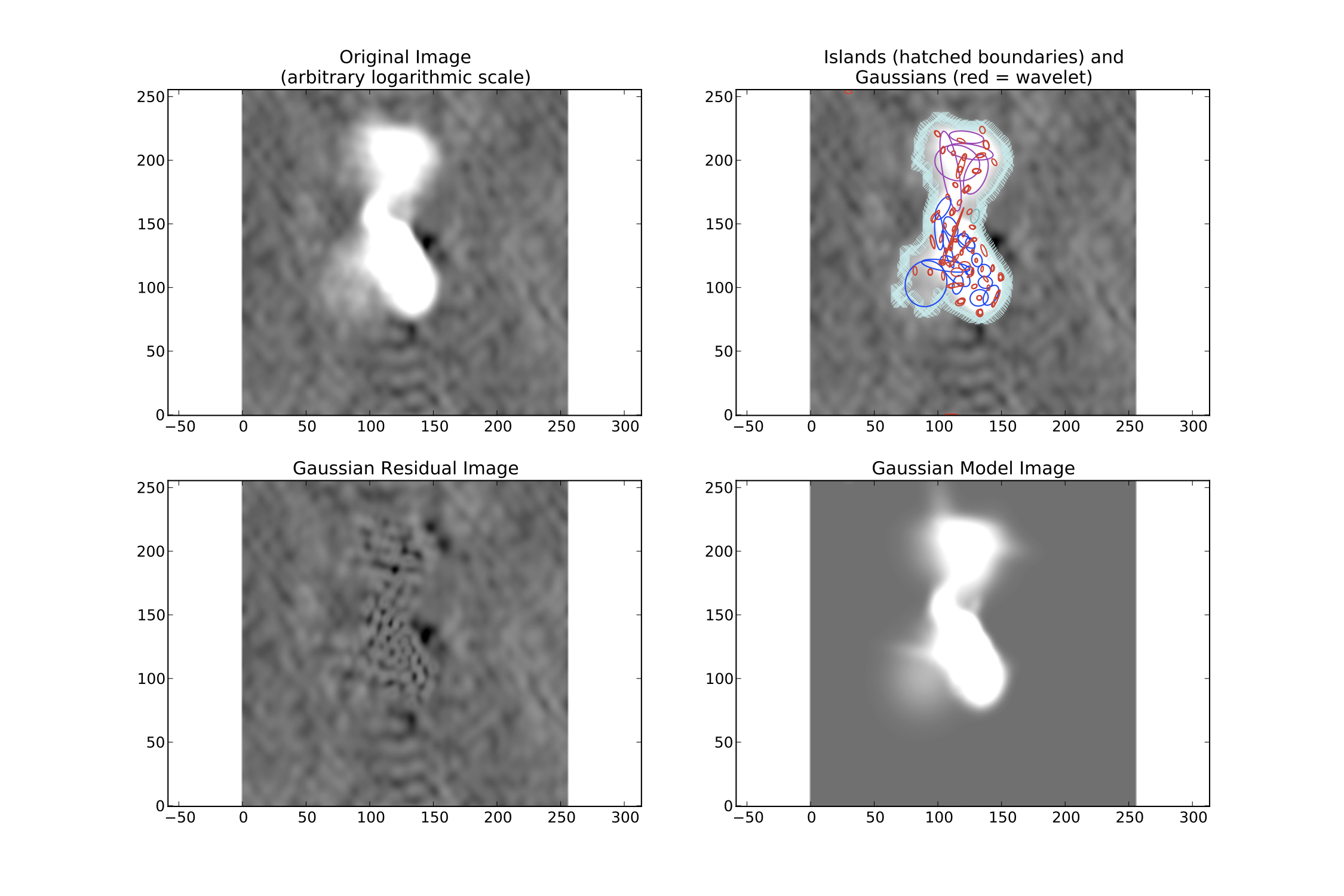
Example fit of an image of Hydra A with rms_map=False, mean_map='zero', flag_maxsize_bm=50 and atrous_do=True. The values of thresh_isl and thresh_pix were adjusted before fitting (by setting interactive=True) to obtain an island that enclosed all significant emission.
Scripting example
You can use the complete functionality of PyBDSF within Python scripts (see Scripting PyBDSF for details). Scripting can be useful, for example, if you have a large number of images or if PyBDSF needs to be called as part of an automated reduction. Below is a short example of using PyBDSF to find sources in a number of images automatically. In this example, the best reduction parameters were determined beforehand for a representative image and saved to a PyBDSF save file using the tput command (see Commands for details).
# pybdsf_example.py
#
# This script fits a number of images automatically, writing out source
# catalogs and residual and model images for each input image. Call it
# with "python pybdsf_example.py"

import bdsf

# Define the list of images to process and the parameter save file
input_images = ['a2597.fits', 'a2256_1.fits', 'a2256_2.fits',
                 'a2256_3.fits', 'a2256_4.fits', 'a2256_5.fits']
save_file = 'a2256.sav'

# Now loop over the input images and process them
for input_image in input_images:

    if input_image == 'a2597.fits':
        # For this one image, run with different parameters.
        # Note that the image name is the first argument to
        # process_image:
        img = bdsf.process_image(input_image, rms_box=(100,20))

    else:
        # For the other images, use the 'a2256.sav` parameter save file.
        # The quiet argument is used to supress output to the terminal
        # (it still goes to the log file).
        # Note: when a save file is used, it must be given first in the
        # call to process_image:
        img = bdsf.process_image(save_file, filename=input_image, quiet=True)

    # Write the source list catalog. File is named automatically.
    img.write_catalog(format='fits', catalog_type='srl')

    # Write the residual image. File is named automatically.
    img.export_image(img_type='gaus_resid')

    # Write the model image. Filename is specified explicitly.
    img.export_image(img_type='gaus_model', outfile=input_image+'.model')
Using SAMP interoperability
PyBDSF supports SAMP (Simple Application Messaging Protocol) to provide interoperability to other applications, such as TOPCAT [1], ds9 [2], and Aladin [3]. To use this functionality, a SAMP hub must be running (both TOPCAT and Aladin come with SAMP hubs). Below is an example of using PyBDSF with TOPCAT. In this example, it is assumed that an image has already been processed with process_image.
BDSF [1]: process_image('VLSS.fits')
...
At this point, make sure that TOPCAT is started and its SAMP hub is running (activated by clicking the “Attempt to connect to SAMP hub” icon in the lower right-hand corner and selecting “Start internal hub”). Next, we send the PyBDSF source list to TOPCAT with write_catalog:
BDSF [2]: inp write_catalog

BDSF [3]: outfile='SAMP'

BDSF [4]: go
---------> go()
--> Table sent to SAMP hub.
TOPCAT should automatically load the table. Double-click on the table name in TOPCAT to open the table viewer. We can use now the show_fit task to highlight the table row that corresponds to a source of interest. To do this, we start show_fit with broadcast = True:
BDSF [6]: show_fit(broadcast=T)
========================================================================
NOTE -- With the mouse pointer in plot window:
  Press "i" ........ : Get integrated flux densities and mean rms
                       values for the visible portion of the image
  Press "m" ........ : Change min and max scaling values
  Press "n" ........ : Show / hide island IDs
  Press "0" ........ : Reset scaling to default
  Click Gaussian ... : Print Gaussian and source IDs (zoom_rect mode,
                       toggled with the "zoom" button and indicated in
                       the lower right corner, must be off)
________________________________________________________________________
Now, clicking on a Gaussian will highlight the row corresponding to the source to which the Gaussian belongs. Gaussian catalogs (i.e., made with catalog_type='gaul' in write_catalog) are also supported (and may be used simultaneously in TOPCAT with source catalogs).
Images can be sent to ds9 or Aladin using the export_image task in the same way (with outfile = 'SAMP'). Furthermore, if an image was sent, clicking on a Gaussian in the show_fit window will tell ds9 or Aladin to center their view on the coordinates of the Gaussian’s center.
Footnotes